
You paste a position into a solver. A few milliseconds later it tells you column 5 wins, column 3 draws, and everything else loses.
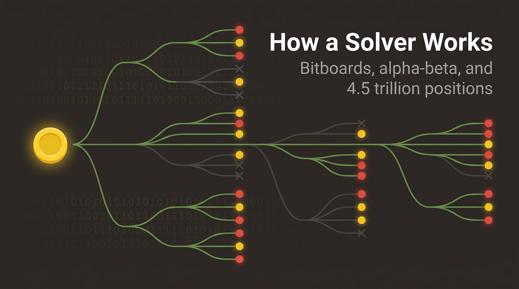
That answer is not an estimate. It is not a rating, a confidence score, or a neural network's best guess. It is the true value of the position, the same value you would get by playing out every possible continuation to the last disc.
So how does it get there that fast?
We built one. It lives behind the engine and the position solver on this site, and it is a few hundred lines of C++ that most people would not recognise as a board game. Here is what is actually inside it.
The Problem Is Size
Connect Four is solved. John Tromp counted the legal positions on a 7x6 board: 4,531,985,219,092. Roughly 4.5 trillion.
A naive program that just tries every move, then every reply, then every reply to that, would have to walk a game tree far larger than that number, because the same position gets reached by many different move orders. Victor Allis put the loose upper bound at about 7.1 x 10^13 board states in his 1988 thesis.
At a billion positions per second, brute force takes hours per query. Nobody waits hours.
Every technique below exists for one reason: to answer the same question while looking at a few million positions instead of a few trillion.
Step 1: The Board Is Two Numbers
The first thing a fast solver throws away is the board.
No 6x7 array. No grid of cells. A position is two 64-bit integers:
position- the discs belonging to the player whose turn it ismask- every occupied square, both colours
That is it. The opponent's discs are position ^ mask, which is one instruction.
The bits are laid out 7 per column on a 6-row board. Six real squares plus one sentinel bit on top:
row 6    5   12   19   26   33   40   47
row 5    4   11   18   25   32   39   46
row 4    3   10   17   24   31   38   45
row 3    2    9   16   23   30   37   44
row 2    1    8   15   22   29   36   43
row 1    0    7   14   21   28   35   42
       col1 col2 col3 col4 col5 col6 col7
Bits 6, 13, 20, 27, 34, 41 and 48 are the sentinels. They are never played. They exist so that arithmetic carrying out of one column cannot leak into the next.
That layout makes the whole game cheap. Dropping a disc in a column is three operations:
position ^= mask;                    // hand the turn to the opponent
mask |= mask + BOT_MASK[col];        // carry finds the lowest empty square
++moves;
The second line is the trick. Adding the bottom bit of a column to the mask makes the carry ripple up through the discs already there and land on exactly the first empty square. Gravity, for free, as a side effect of binary addition. That is why the sentinel row exists: without it, a full column would carry into its neighbour.
Step 2: Checking for Four in a Row Without Looking
The next thing to make fast is the win check, because the search runs it constantly.
You could loop over every square and count in four directions. A bitboard does it with shifts. Four in a row in a given direction means four bits set at a constant stride. Shift, AND, shift again, AND:
uint64_t m = pos & (pos >> 7);       // horizontal pairs
if (m & (m >> 14)) return true;      // two pairs, 7 apart = four in a row
Stride 7 is horizontal. Stride 1 is vertical. Stride 6 and stride 8 are the two diagonals. Four directions, eight instructions, no branches, no loops, and it checks all 69 possible four-in-a-rows at once.
The same idea gives you something more useful than "did I win". By shifting the position around and looking for the gaps, you get a mask of every empty square that would complete four for a player. That is a threat map, computed as a single integer, and the rest of the solver is built on it.
If you have read the odd/even threat guide, that mask is the same object you build in your head at the board. The solver just gets it in one instruction.
Step 3: The Search Is Negamax With Alpha-Beta
Now the actual searching.
The base algorithm is minimax: I pick the move that maximises my score, assuming you then pick the move that minimises it, and so on to the end of the game. Negamax is minimax written once instead of twice, using the fact that your best score is the negative of my best score from the same position.
Alpha-beta pruning is what makes it usable. The search carries two bounds: alpha, the best score the searching player has already guaranteed, and beta, the best the opponent has already guaranteed. The moment a branch proves it cannot beat what has already been found, the search abandons it without looking at the rest.
Concretely: you are checking your opponent's replies to a candidate move. The first reply you try already wins for them. There is no reason to check their other six replies. That move is refuted, cut it, move on.
This is not an approximation. Alpha-beta returns exactly the same answer as full minimax. It just skips the branches whose answers cannot change the result. Allen and Allis both leaned on it in 1988, and it is still the backbone of every serious Connect Four solver.
Step 4: The Order You Try Moves Decides Everything
Alpha-beta only cuts when it finds a good move early. Try the best move first and you prune almost everything below it. Try it last and you have searched the whole subtree before you get there.
So move ordering is not a polish step. It is the single largest performance lever in the solver.
Two heuristics do the work. The first is static: try columns from the centre outward, in the order 4, 3, 5, 2, 6, 1, 7. This is the same reason column 4 is the only winning first move - central squares sit on more of the 69 possible lines, so central moves are more often best, so they cut sooner.
The second is dynamic and better. Before recursing, score each candidate move by how many new threats it creates, using the threat mask from step 2, then sort descending. A move that opens two new winning squares is far more likely to be the refutation than one that opens none.
In our solver these two combine and the effect is not subtle. The same search that would take minutes with random move ordering finishes in single-digit milliseconds.
Step 5: Refusing to Search Losing Moves
There is a class of move you never have to search at all.
If your opponent has an immediate winning square available right now, you have exactly one legal idea: block it. Searching the other six columns is pure waste, they all lose. And if the opponent has two immediate winning squares, you are lost no matter what, so the search returns immediately without expanding anything.
There is a subtler version. Never play directly underneath a square that wins for your opponent. You fill the square below, they drop on top, game over. The solver computes the opponent's threat mask, shifts it down one bit, and removes those squares from the candidate list before the search even starts.
If that rule sounds familiar, it should. It is the same "do not open your opponent's square" discipline that decides the endgame, except the solver applies it at every node of a million-node search without ever getting bored.
Step 6: The Transposition Table
Move order 4, 3, 5 reaches the same board as 5, 3, 4. Move order 3, 4, 5 reaches it too. The game tree is not a tree at all, it is a graph, and the naive search re-solves the same positions over and over.
A transposition table is a big hash table that remembers what a position was worth. Ours holds 8,388,593 entries, a prime just under 2^23, and the index is simply the position key modulo that prime.
The key itself is a nice piece of bitboard trickery: position + mask. Adding the mask to the current player's discs shifts every column's occupancy up by one bit, which produces a value that uniquely identifies both the shape of the board and whose discs are whose. One addition, one 64-bit key.
Each entry stores a bound rather than an exact score, because alpha-beta often proves "this is at most X" or "this is at least X" without pinning down the true value. On a hit, the stored bound tightens alpha or beta, and quite often that alone is enough to cut the branch without searching a single child.
The table is reused across queries, so the second position you solve is faster than the first.
Step 7: Binary Search on the Answer
The last trick is the least intuitive one.
Instead of asking "what is this position worth", which forces a wide search, the solver asks a yes/no question: "is this position worth more than X?" A null-window search, where alpha and beta are adjacent integers, prunes far more aggressively than a wide one because almost every branch fails one side of the window immediately.
Then it binary-searches X. Scores in Connect Four live in a small range, roughly -18 to 18, so about five null-window searches pin the exact value. Five cheap searches beat one expensive one, by a lot.
The score that comes out is not arbitrary. A positive score means the player to move wins, negative means they lose, zero is a draw. The magnitude is how fast: the formula is (43 - total_discs_at_the_end) / 2, so a score of 2 means the win lands with 39 discs on the board, and the maximum score of 18 means the game ends with only 7 discs on the board, the fastest win the game allows. Higher is sooner.
That is why our engine can tell you not just that you are winning, but that you are winning in 11 more moves and that the other column only wins in 19.
The One Thing Solvers Still Cannot Do Fast
The empty board.
Everything above works beautifully from move 8 onward. Our solver averages about 5.7 ms per position on mid-game boards, around 9 million nodes per second, roughly 28x faster than the TypeScript implementation it replaced.
Hand it the empty 7x6 board and it will sit there. So will Pascal Pons' reference solver, whose techniques ours is built on. Alpha-beta needs threats to prune against, and on an empty board there are none for a dozen plies. The search fans out with almost no cuts.
The fix is not a better algorithm. It is an opening book: a precomputed table of the first several plies, solved once offline over many CPU hours, then looked up instantly forever after. Allis' VICTOR program spent around 1000 CPU hours in 1988 to do this work, 350 of them on the four main winning variations. Tromp went further between 1993 and 1995 and computed the value of every legal position outright.
Modern solvers do not re-derive that. They inherit it. The clever part of a fast solver is the middlegame, and the opening comes out of a book somebody else paid for in 1988.
What This Means at the Board
You are not going to run alpha-beta in your head. But three of the solver's ideas are directly transferable, and strong players already use them.
Search the forcing moves first. The solver prunes by trying the move that creates the most threats before anything else. When you are calculating, do the same. Check the moves that force a reply before the quiet ones, because if one of them works you are done thinking.
Prune losing moves before you calculate. The solver deletes every square that sits under an opponent winning square, then searches what is left. That is a checklist, not a calculation. Run it first and your real thinking starts from three candidate columns instead of seven.
Remember positions, not lines. The transposition table exists because the same board arrives by many routes. Your pattern memory does the same job. Learning what a double threat shape is worth beats memorising the move order that produced it.
Try It
The fastest way to understand a solver is to argue with one.
Take a position you thought was fine and run it through the solver. Then take a game you lost and review it move by move, watching for the ply where the evaluation flipped. It is almost never where you think it was.
Then go play the engine at full strength. It is the same code described above, and it will not miss.
If you want the theory behind the answers it gives you, start with what "solved" actually means, then the parity counting that decides most of the positions the solver scores as wins.